Interactive online version:
3D Radiation Emitter
This notebook demonstrates how to create a 3D radiation emitter from IMAS radiation IDS.
The example test data was calculated by JOREK for an ITER disruption scenario.
[1]:
import numpy as np
import ultraplot as uplt
from imas import DBEntry
from raysect.optical import World
from rich import print as rprint
from rich.table import Table
from cherab.core.math import sample3d_grid
from cherab.imas.datasets import iter_jorek
from cherab.imas.emitter import load_radiation_emitter
# Set dark background for plots
uplt.rc.style = "dark_background"
TOGW = 1e-9 # [W] -> [GW]
Retrieve ITER JOREK sample data
[2]:
path = iter_jorek()
Create 3D radiation emitter from IMAS IDS
[3]:
world = World()
emitter = load_radiation_emitter(
path,
"r",
time=0.0042853,
parent=world,
interpolator_cache="disk",
)
17:13:52 INFO Parsing data dictionary version 4.1.1 @dd_zip.py:89
17:13:53 INFO Parsing data dictionary version 4.0.0 @dd_zip.py:89
/home/runner/work/imas/imas/src/cherab/imas/emitter/radiation.py:122: RuntimeWarning: The 'get_slice' method is not implemented for the URI '/home/runner/.cache/cherab/imas/iter_disruption_113112_1.nc'. Falling back to 'get' and re-slicing via the IMAS memory backend.
radiation_ids = get_ids_time_slice(
Visualize the emitter in 2D
Sample 2D visualization of the radiation function at all toroidal angles.
[4]:
R_MIN, R_MAX = 4.0, 8.5
Z_MIN, Z_MAX = -4.5, 4.4
RES = 0.01 # resolution of grid in [m]
n_r = round((R_MAX - R_MIN) / RES) + 1
n_z = round((Z_MAX - Z_MIN) / RES) + 1
dr, dz = (R_MAX - R_MIN) / (n_r - 1), (Z_MAX - Z_MIN) / (n_z - 1)
# (r, z) coordinates at phi=0
r_pts = np.linspace(R_MIN, R_MAX, n_r, endpoint=True)
z_pts = np.linspace(Z_MIN, Z_MAX, n_z, endpoint=True)
# Toroidal angles to sample the radiation function at
n_phi = 64
d_phi = 360 / n_phi
eps = 1e-6 # small offset to avoid sampling at exactly 0 and 360 degrees
phis = np.linspace(0 + d_phi + eps, 360 + d_phi - eps, n_phi + 1, endpoint=True)
[5]:
n_phi = len(phis)
rad = np.zeros((n_r, n_z, n_phi), dtype=float)
for i, j, k in np.ndindex(n_r, n_z, n_phi):
rad[i, j, k] = emitter.material.radiation_function(
r_pts[i] * np.cos(np.deg2rad(phis[k])),
r_pts[i] * np.sin(np.deg2rad(phis[k])),
z_pts[j],
)
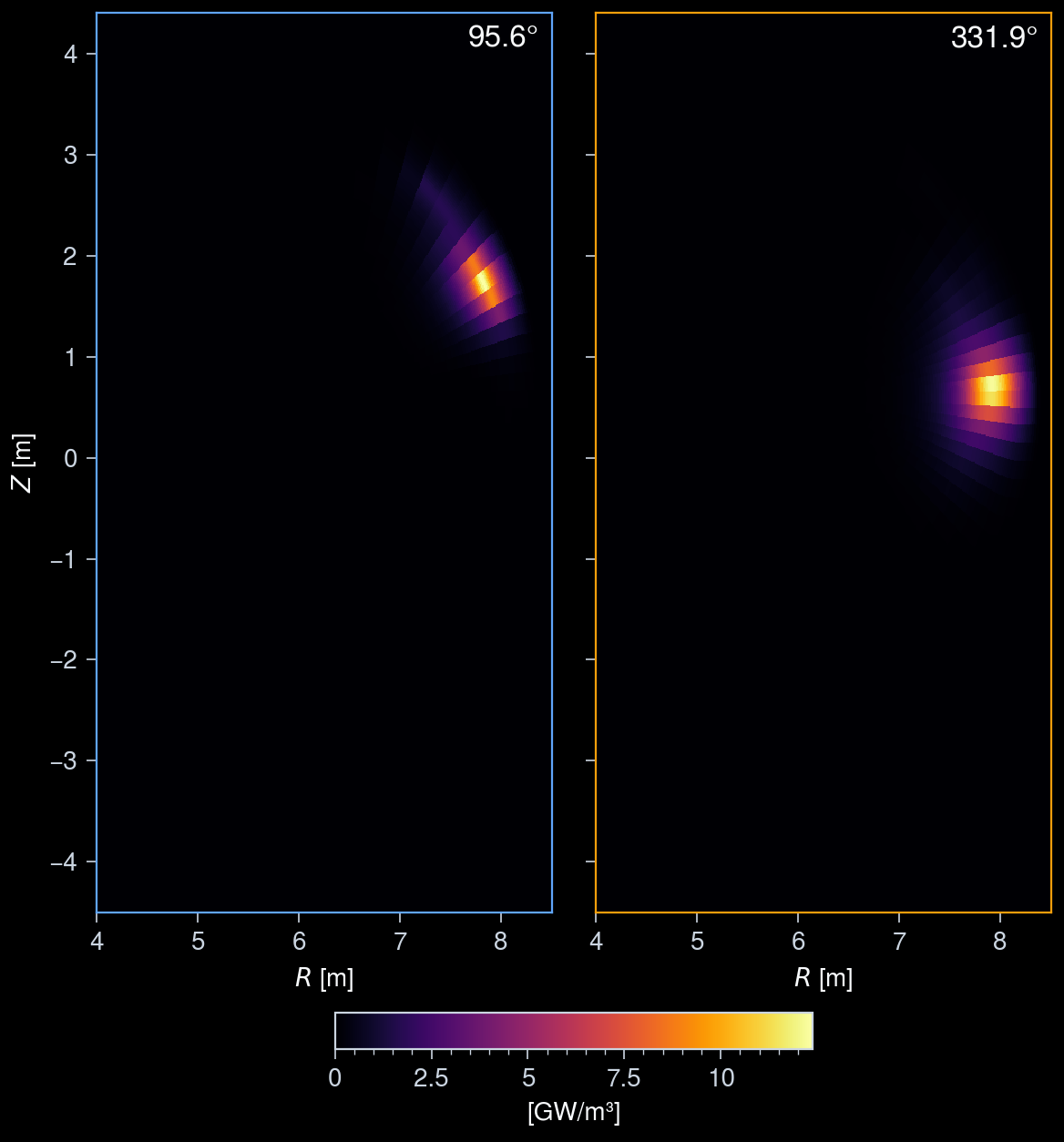
Cross-sectional view of the radiation
2D poloidal cross-sections of the radiation function at two toroidal angles.
[6]:
phi_selected = [95, 330] # toroidal angles to visualize
# Get the maximum value
vmax = -np.inf
for phi in phi_selected:
i_phi = np.argmin(np.abs(phis - phi))
vmax = max(vmax, np.max(rad[:, :, i_phi] * TOGW))
fig, axs = uplt.subplots(ncols=len(phi_selected), spanx=False)
for i, phi in enumerate(phi_selected):
i_phi = np.argmin(np.abs(phis - phi))
im = axs[i].pcolormesh(
r_pts,
z_pts,
rad[:, :, i_phi].T * TOGW,
shading="auto",
cmap="inferno",
discrete=False,
vmax=vmax,
vmin=0,
)
axs[i].format(
axesedgecolor=f"C{i}",
urtitle=f"{phis[i_phi]:.1f}°",
titleborder=False,
aspect="equal",
xlabel="$R$ [m]",
ylabel="$Z$ [m]",
)
fig.colorbar(
im,
ax=axs,
loc="b",
label="[GW/m³]",
shrink=0.5,
tickminor=True,
);
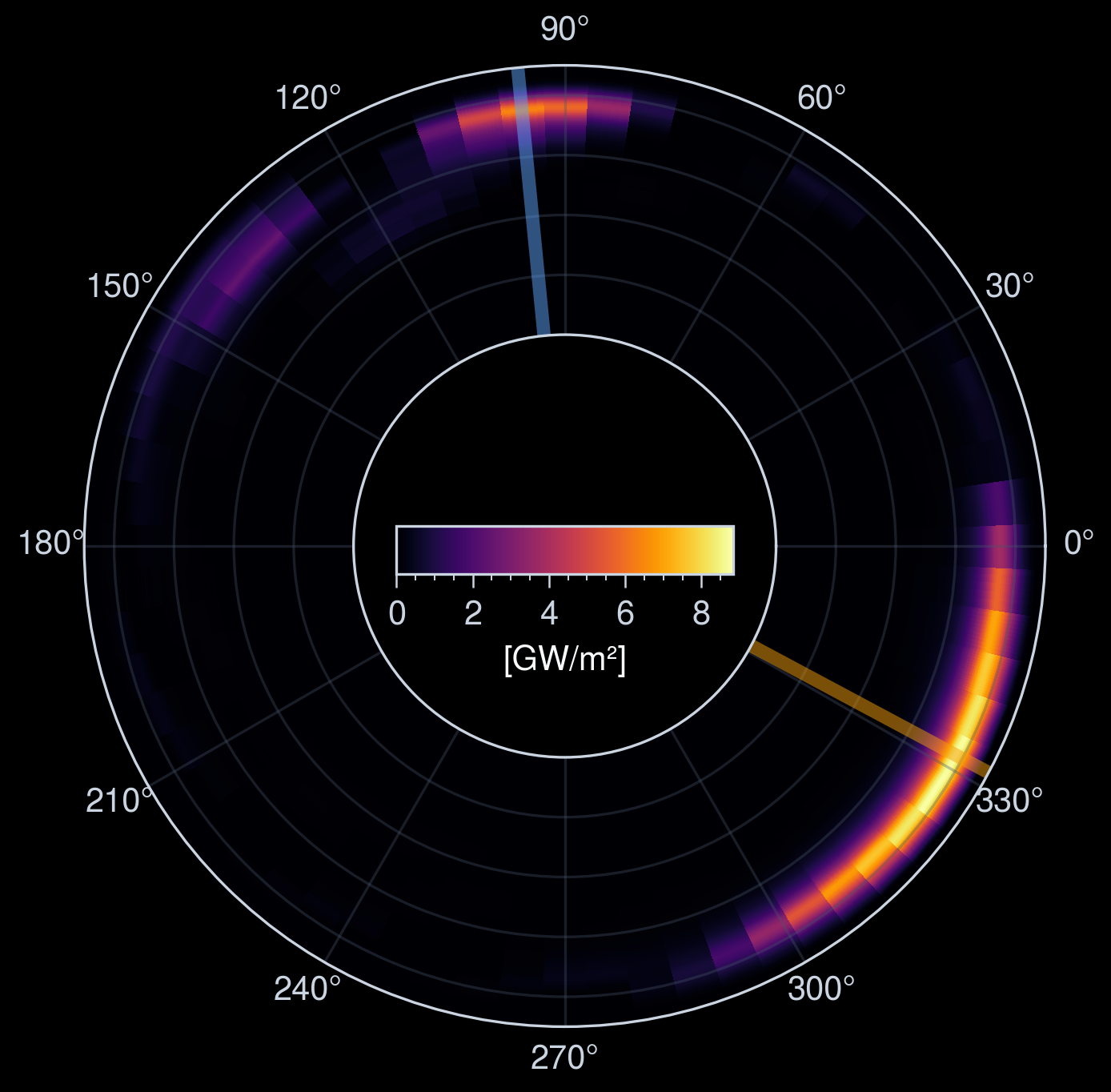
Z-integrated X-Y projection
The radiation distribution is integrated along the z-axis and projected onto the X-Y plane.
Each toroidal angle at which the cross-section was plotted above is also shown as a colored line in the X-Y projection.
[7]:
fig, ax = uplt.subplots(
proj="polar",
dpi=150,
refwidth=4,
)
im = ax.pcolormesh(
np.deg2rad(phis),
r_pts,
rad.sum(axis=1) * TOGW * dz,
shading="auto",
cmap="inferno",
discrete=False,
vmin=0,
)
fig.colorbar(
im,
ax=ax,
label="[GW/m²]",
loc="b",
shrink=0.35,
ticks=2,
tickminor=True,
orientation="horizontal",
pad=-15,
)
for i, phi in enumerate(phi_selected):
ax.axvline(
np.deg2rad(phis[np.argmin(np.abs(phis - phi))]),
color=uplt.set_alpha(f"C{i}", 0.5),
lw=4,
)
ax.format(
rmin=r_pts.min(),
rmax=r_pts.max(),
rformatter="none",
r0=r_pts.min() / r_pts.max(),
thetalocator=30,
rlabelpos=0,
rlines=1,
)
Visualize the emitter in 3D
Resample the radiation function between the toroidal angle 270° and 360° (quarter of the torus) in (X, Y, Z) coordinates and visualize the result in 3D.
To plot 3D data, we use the plotly library. The 3D radiation distribution is visualized as a volume rendering.
[8]:
import plotly.graph_objects as go
from plotly import io
io.renderers.default = "notebook"
[9]:
dr = dz = 10e-2
x_pts = np.arange(0, R_MAX, dr)
y_pts = np.arange(0, -R_MAX, -dr)
z_pts = np.arange(Z_MIN, Z_MAX, dz)
X, Y, Z = np.meshgrid(x_pts, y_pts, z_pts)
rad_xyz = np.zeros((len(x_pts), len(y_pts), len(z_pts)), dtype=float)
for i, j, k in np.ndindex(len(x_pts), len(y_pts), len(z_pts)):
rad_xyz[i, j, k] = emitter.material.radiation_function(x_pts[i], y_pts[j], z_pts[k])
[10]:
fig = go.Figure(
data=go.Volume(
x=X.flatten(),
y=Y.flatten(),
z=Z.flatten(),
value=rad_xyz.flatten(),
isomin=1e8,
isomax=rad_xyz.max(),
opacity=0.1, # needs to be small to see through all surfaces
surface_count=21, # needs to be a large number for good volume rendering
)
)
fig.update_layout(
scene=dict(
xaxis_title="X [m]",
yaxis_title="Y [m]",
zaxis_title="Z [m]",
aspectmode="data",
),
margin=dict(l=0, r=0, b=0, t=0),
template="plotly_dark",
)