This page was generated from
docs/notebooks/radiation/grid_3d.ipynb.
Interactive online version: .
Download notebook.
.
Download notebook.
Interactive online version:
3D Grid Visualization
This notebook demonstrates how to load and visualize a 3-D grid from Generalized Grid Description (GGD) in IMAS.
The example test data was calculated by JOREK for an ITER disruption scenario.
[1]:
import numpy as np
import ultraplot as uplt
from imas import DBEntry
from rich import print as rprint
from rich.table import Table

from cherab.imas.datasets import iter_jorek
from cherab.imas.ids.common import get_ids_time_slice
from cherab.imas.ids.common.ggd import load_grid

# Set dark background for plots
uplt.rc.style = "dark_background"
Retrieve ITER JOREK sample data
[2]:
path = iter_jorek()
Downloading file 'iter_disruption_113112_1.nc' from 'doi:10.5281/zenodo.17062699/iter_disruption_113112_1.nc' to '/home/runner/.cache/cherab/imas'.
Retrieve the GGD data belonging to the radiation IDS.
[3]:
with DBEntry(path, "r") as entry:
    ids = get_ids_time_slice(entry, "radiation")
    grid = load_grid(ids.grid_ggd[0])
17:12:33 INFO     Parsing data dictionary version 4.1.1 @dd_zip.py:89
17:12:33 INFO     Parsing data dictionary version 4.0.0 @dd_zip.py:89
/tmp/ipykernel_3725/3961500530.py:2: RuntimeWarning: The 'get_slice' method is not implemented for the URI '/home/runner/.cache/cherab/imas/iter_disruption_113112_1.nc'. Falling back to 'get' and re-slicing via the IMAS memory backend.
  ids = get_ids_time_slice(entry, "radiation")
Show the grid specification
[4]:
table = Table(show_header=False, title="Grid specification")
table.add_row("Grid name", str(grid.name))
table.add_row("Number Faces", str(grid.num_faces))
table.add_row("Number Toroidal", str(grid.num_toroidal))
table.add_row("Number Cell", str(grid.num_cell))
table.add_row("Shape of vertices array", str(grid.vertices.shape))
table.add_row("Shape of cells array", str(grid.cells.shape))
rprint(table)
           Grid specification
┌─────────────────────────┬─────────────┐
│ Grid name               │ JOREK mesh  │
│ Number Faces            │ 6398        │
│ Number Toroidal         │ 64          │
│ Number Cell             │ 409472      │
│ Shape of vertices array │ (418304, 3) │
│ Shape of cells array    │ (409472, 8) │
└─────────────────────────┴─────────────┘
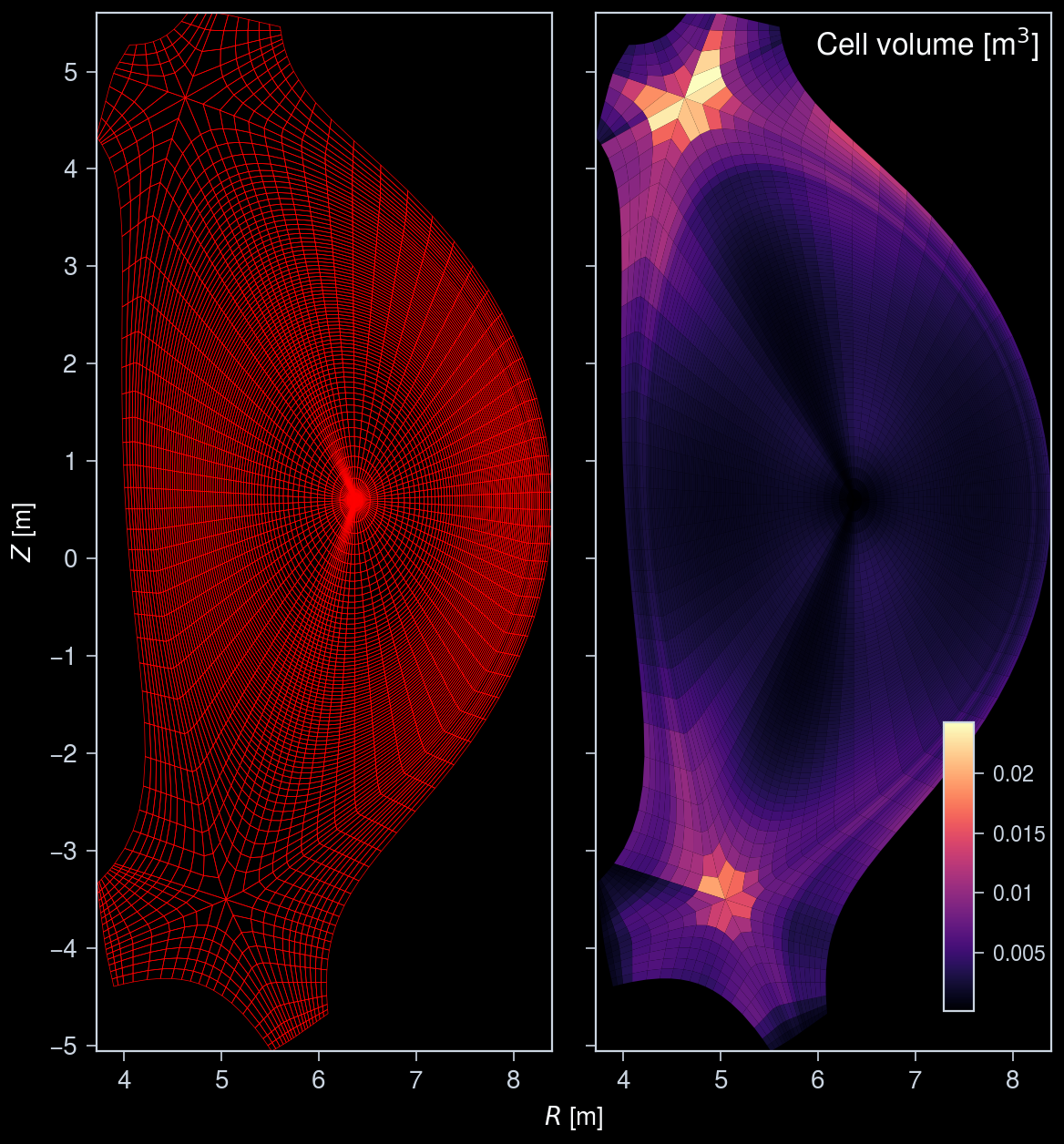
Visualize the cross-section of the grid
Show the grid lines and cell volume map in the poloidal cross-section of the grid.
[5]:
fig, axs = uplt.subplots(ncols=2)
# Plot the grid mesh in 2D cross-section
grid.plot_mesh(ax=axs[0], edgecolor="red")

# Plot the cell volume map in 2D cross-section
ax = grid.plot_mesh(ax=axs[1], data=grid.cell_volume[: grid.num_faces])
ax.collections[0].set_cmap("magma")

ax.colorbar(
    ax.collections[0],
    tickdir="out",
    loc="lr",
    orientation="vertical",
    ticklabelsize="small",
    length=5,
    frame=False,
)
ax.format(
    urtitle="Cell volume [m$^3$]",
    titleborder=False,
)

# Format the axes
axs.format(xlocator=1, ylocator=1)
Plot center points of cells
[6]:
# Extract cell center points for one toroidal slice
cell_centers = grid.cell_centre[: grid.num_faces, :]

# Calculate the (r, z) coordinates
r_coords = np.hypot(cell_centers[:, 0], cell_centers[:, 1])
z_coords = cell_centers[:, 2]

fig, ax = uplt.subplots()

# Plot grid and cell centers in the poloidal cross-section
grid.plot_mesh(
    ax=ax,
    edgecolor="red",
)
ax.scatter(r_coords, z_coords, s=1, c="C0")
ax.format(
    xlocator=1,
    ylocator=1,
)

# Zoom in around divertor region
ix = ax.inset(
    [7.0, -9, 6, 6],
    transform="data",
    zoom_kw={"ec": "grape3", "ls": "--", "lw": 2},
)
grid.plot_mesh(ax=ix, edgecolor="red")
ix.scatter(r_coords, z_coords, s=1, c="C0")
ix.format(
    xlim=(ax.get_xlim()[0], 6.2),
    ylim=(ax.get_ylim()[0], -3.0),
    aspect="equal",
    color="grape9",
    linewidth=1.5,
    ticklabelweight="bold",
    xlocator=1,
    ylocator=1,
    xformatter="none",
    yformatter="none",
    xlabel="",
    ylabel="",
)
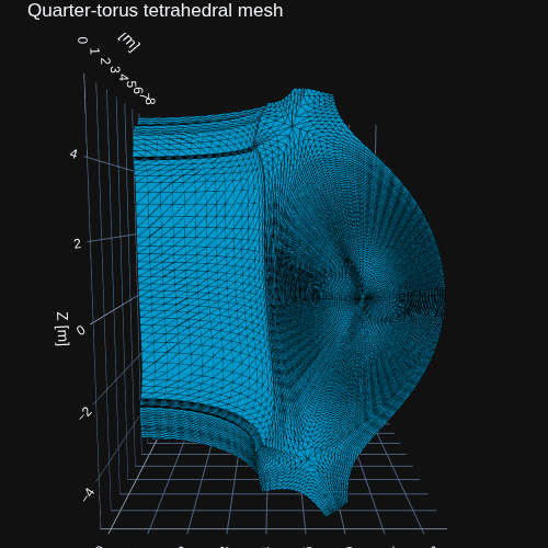
Cut out quarter of the torus
[7]:
grid_cut = grid.subset(np.arange(grid.num_faces * grid.num_toroidal // 4))
Visualize the 3D grid in a quarter of the torus. plotly is used to visualize the tetrahedral mesh in the notebook.
[8]:
import plotly.graph_objects as go
[9]:
tetra = grid_cut.tetrahedra
faces = np.vstack(
    [
        tetra[:, [0, 1, 2]],
        tetra[:, [0, 1, 3]],
        tetra[:, [0, 2, 3]],
        tetra[:, [1, 2, 3]],
    ]
)

# Keep only boundary faces (faces appearing exactly once).
faces_sorted = np.sort(faces, axis=1)
_, inverse, counts = np.unique(faces_sorted, axis=0, return_inverse=True, return_counts=True)
surface_faces = faces[counts[inverse] == 1]

# Build unique boundary edges from boundary triangles.
tri_edges = np.vstack(
    [
        surface_faces[:, [0, 1]],
        surface_faces[:, [1, 2]],
        surface_faces[:, [2, 0]],
    ]
)
boundary_edges = np.unique(np.sort(tri_edges, axis=1), axis=0)

verts = grid_cut.vertices
x, y, z = verts[:, 0], verts[:, 1], verts[:, 2]

# Customize edge appearance here.
edge_color = "black"
edge_width = 1.5

# Convert edge index pairs to line segments separated by NaN for Plotly.
edge_xyz = verts[boundary_edges]
xe = np.column_stack(
    [edge_xyz[:, 0, 0], edge_xyz[:, 1, 0], np.full(len(boundary_edges), np.nan)]
).ravel()
ye = np.column_stack(
    [edge_xyz[:, 0, 1], edge_xyz[:, 1, 1], np.full(len(boundary_edges), np.nan)]
).ravel()
ze = np.column_stack(
    [edge_xyz[:, 0, 2], edge_xyz[:, 1, 2], np.full(len(boundary_edges), np.nan)]
).ravel()

fig = go.Figure(
    data=[
        go.Mesh3d(
            x=x,
            y=y,
            z=z,
            i=surface_faces[:, 0],
            j=surface_faces[:, 1],
            k=surface_faces[:, 2],
            color="deepskyblue",
            flatshading=True,
            hoverinfo="skip",
            showscale=False,
            name="Surface",
        ),
        go.Scatter3d(
            x=xe,
            y=ye,
            z=ze,
            mode="lines",
            line=dict(color=edge_color, width=edge_width),
            name="Surface boundary",
            hoverinfo="skip",
        ),
    ]
)

fig.update_layout(
    title="Quarter-torus tetrahedral mesh",
    width=500,
    height=500,
    scene=dict(
        xaxis_title="X [m]",
        yaxis_title="Y [m]",
        zaxis_title="Z [m]",
        aspectmode="data",
    ),
    margin=dict(l=0, r=0, b=0, t=30),
    scene_camera=dict(
        eye=dict(x=0.0, y=-2.0, z=0.25),
    ),
    template="plotly_dark",
)
fig.show(
    renderer="png",
)